Source: Dominique R. Bollino1, Eric A. Legenzov2, Tonya J. Webb1
1 Département de microbiologie et d’immunologie, University of Maryland School of Medicine et Marlene and Stewart Greenebaum Comprehensive Cancer Center, Baltimore, Maryland 21201
2 Center for Biomedical Engineering and Technology, University of Maryland School of Medicine, Baltimore, Maryland 21201
La microscopie par fluorescence confocale est une technique d’imagerie qui permet une résolution optique accrue par rapport à la microscopie d’épifluorescence « à champ large » classique. Les microscopes confocals sont capables d’obtenir une meilleure résolution optique x-y grâce à la « numérisation laser » – généralement un ensemble de miroirs à tension contrôlée (miroirs de galvanomètre ou de « galvo ») qui dirigent l’éclairage laser à chaque pixel du spécimen à la fois. Plus important encore, les microscopes confocals atteignent une résolution z-axiale supérieure en utilisant un sténopé pour enlever la lumière de mise au point provenant d’endroits qui ne sont pas dans le z-plan étant numérisé, permettant ainsi au détecteur de recueillir des données à partir d’un z-plan spécifié. En raison de la haute résolution Z réalisable dans la microscopie confocale, il est possible de recueillir des images à partir d’une série de z-planes (également appelé z-stack) et de construire une image 3D à travers un logiciel.
Avant de discuter du mécanisme d’un microscope confocal, il est important de considérer comment un échantillon interagit avec la lumière. La lumière est composée de photons, des paquets d’énergie électromagnétique. Un photon empiéchant sur un échantillon biologique peut interagir avec les molécules qui composent l’échantillon de l’une des quatre façons : 1) le photon n’interagit pas et passe à travers l’échantillon; 2) le photon est réfléchi/dispersé; 3) le photon est absorbé par une molécule et l’énergie absorbée est libérée sous forme de chaleur par des processus collectivement connus sous le nom de carie non radiative; et 4) le photon est absorbé et l’énergie est alors rapidement réémise en tant que photon secondaire par le processus connu sous le nom de fluorescence. Une molécule dont la structure permet l’émission de fluorescence est appelée fluorophore. La plupart des échantillons biologiques contiennent des fluorophores endogènes négligeables; par conséquent, les fluorophores exogènes doivent être utilisés pour mettre en évidence les caractéristiques d’intérêt dans l’échantillon. Pendant la microscopie de fluorescence, l’échantillon est éclairé avec la lumière de la longueur d’onde appropriée pour l’absorption par le fluorophore. Lors de l’absorption d’un photon, un fluorophore est dit être «excité» et le processus d’absorption est appelé «excitation». Lorsqu’un fluorophore abandonne l’énergie sous la forme d’un photon, le processus est connu sous le nom d’« émission », et le photon émis est appelé fluorescence.
Le faisceau lumineux utilisé pour exciter un fluorophore est focalisé par la lentille objective d’un microscope et converge à un « point focal » où il est focalement focal. Au-delà du point focal, la lumière diverge à nouveau. Les poutres entrantes et sortantes peuvent être visualisées comme une paire de cônes touchant au point focal (voir la figure 1, panneau gauche). Le phénomène de diffraction impose une limite à la façon dont étroitement un faisceau de lumière peut être concentré – le faisceau se concentre réellement à un endroit de taille finie. Deux facteurs déterminent la taille de la tache focale : 1) la longueur d’onde de la lumière, et 2) la capacité de collecte de lumière de la lentille objective, qui se caractérise par son ouverture numérique (NA). Le «spot» focal s’étend non seulement dans le plan x-y, mais aussi dans la direction z, et est en réalité un volume focal. Les dimensions de ce volume focal définissent la résolution maximale réalisable par l’imagerie optique. Bien que le nombre de photons soit le plus grand dans le volume focal, les chemins de lumière conique au-dessus et au-dessous de la mise au point contiennent également une densité plus faible de photons. N’importe quel fluorophore dans le chemin de lumière peut ainsi être excité. Dans la microscopie conventionnelle (à champ large), les émissions des fluorophores au-dessus et au-dessous du plan focal contribuent à la fluorescence hors foyer (un « fond brumeux »), ce qui réduit la résolution et le contraste de l’image, comme le montre la figure 1, le cube rouge représentant l’émission de fluorophore au-dessus du plan focal (étoile rouge) qui a comme conséquence la fluorescence hors-focus (en haut à droite). Ce problème est amélioré dans la microscopie confocale, en raison de l’utilisation d’un trou d’épingle. (figure 2, en bas à droite). Tel que représenté à la figure 3, le trou d’épingle permet aux émissions provenant du point focal d’atteindre le détecteur (à gauche), tout en empêchant la fluorescence hors foyer (à droite) d’atteindre le détecteur, améliorant ainsi à la fois la résolution et le contraste.
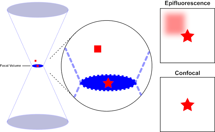
Figure 1. Résolution optique de l’épifluorescence par rapport à la microscopie confocale. Veuillez cliquer ici pour voir une version plus grande de ce chiffre.
Le faisceau lumineux utilisé pour exciter un fluorophore est focalisé par la lentille objective d’un microscope et converge à un volume focal, puis diverge (à gauche). L’étoile rouge représente le plan focal d’un échantillon qui est représenté tandis que le carré rouge représente l’émission de fluorophore au-dessus du plan focal. Lors de la capture d’une image de cet échantillon à l’aide d’un microscope épifluorescent, l’émission du carré rouge flou sera visible et contribuera à un « fond brumeux » (en haut à droite). Les microscopes confocals ont un trou d’épingle qui empêche la détection de la lumière émise à l’extérieur du plan focal, éliminant le « fond brumeux » (en bas à droite).

Figure 2. Effet de trou d’épingle dans la microscopie confocale. Veuillez cliquer ici pour voir une version plus grande de ce chiffre.
Bien que l’intensité la plus élevée de la lumière d’excitation soit au point focal de la lentille (gauche, ovale rouge), d’autres parties de l’échantillon ne se trouve pas dans le point focal (droite, étoile rouge) obtiendront la lumière et la fluoresce. Afin d’éviter que la lumière émise par ces régions floues n’atteigne le détecteur, un écran muni d’un sténopé est présent devant le détecteur. Seule la lumière dans le foyer (à gauche) émise par le plan focal est capable de traverser le sténopé et d’atteindre le détecteur. La lumière hors foyer (à droite) est bloquée avec le sténopé et n’atteint pas le détecteur.
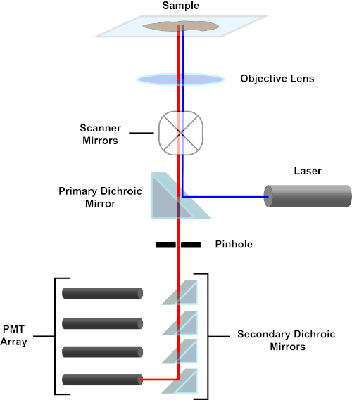
Figure 3. Principaux composants d’un microscope à balayage laser confocal. Veuillez cliquer ici pour voir une version plus grande de ce chiffre.
Par souci de simplicité, la description mécaniste d’un microscope confocal sera limitée à celle du Nikon Eclipse Ti A1R. Bien qu’il puisse y avoir des différences techniques mineures entre les différents microscopes confocal, l’A1R sert bien comme un bon modèle pour décrire la fonction de microscope confocal. Le faisceau lumineux d’excitation, produit par un tableau de lasers à diodes, est reflété par le miroir dichroïque primaire dans l’objectif, qui concentre la lumière sur le spécimen en cours d’image. Le miroir dichroïque primaire réfléchit sélectivement la lumière d’excitation tout en permettant à la lumière à d’autres longueurs d’onde de passer à travers. La lumière rencontre alors les miroirs de balayage qui balaient le faisceau lumineux à travers le spécimen d’une manière x-y, illuminant un seul (x,y) pixel à la fois. La fluorescence émise par les fluorophores au pixel lumineux est recueillie par l’objectif et passe à travers le miroir dichroïque primaire pour atteindre un tableau de tubes photomultiplicateurs (PMT). Les miroirs dichroiques secondaires dirigent la lumière d’émission vers le PMT approprié. La lumière d’excitation dispersée par l’échantillon dans l’objectif est réfléchie par le miroir dichroïque primaire vers le spécimen, et donc empêchée d’entrer dans la détection voie légère et d’atteindre les PMT (voir la figure 3). Cela permet de quantifier la fluorescence relativement faible sans contamination par la lumière dispersée du faisceau lumineux d’excitation, qui est généralement des ordres de grandeur plus intenses que la fluorescence. Parce que le sténopé bloque la lumière de l’extérieur du volume focal, la lumière arrivant au détecteur provient d’un étroit, sélectionné z-plan. Par conséquent, les images peuvent être recueillies à partir d’une série de z-planesadjacents; cette série d’images est souvent appelée « z-stack ». En utilisant le logiciel approprié, une pile zpeut être traitée pour générer une image 3D du spécimen. Un avantage particulier de la microscopie confocale est la capacité de distinguer la localisation subcellulaire de la coloration. Par exemple, la différenciation entre la coloration de membrane de la coloration intracellulaire, qui est très provocante avec la microscopie conventionnelle d’épifluorescence (1, 2, 3).
La préparation de l’échantillon est une facette importante de l’imagerie confocale. Une force des techniques de microscopie optique est la flexibilité d’imager des cellules vivantes ou fixes. Lorsque vous tentez de produire des images 3D, en raison du nombre d’images qui doivent être acquises pour une z-pile, la difficulté de maintenir la santé cellulaire, et le mouvement des cellules vivantes et de leurs organites, l’utilisation de cellules fixes est typique. La procédure pour fixer et tacher des cellules pour la fluorescence confocale est semblable à celle conventionnellement employée dans l’immunofluorescence. Après la culture dans les diapositives de chambre ou sur les couvertures, les cellules sont fixées à l’aide de paraformaldéhyde pour préserver la morphologie cellulaire. La liaison non spécifique d’anticorps est bloquée utilisant l’albumine bovine de sérum, le lait, ou le sérum normal. Afin de maintenir la spécificité des anticorps secondaires, la solution utilisée ne doit pas provenir de la même espèce dans laquelle les anticorps primaires ont été générés. Les cellules sont incubées avec des anticorps primaires qui lient l’antigène d’intérêt. Lors de l’étiquetage de plusieurs cibles cellulaires, les anticorps primaires doivent être dérivés d’une espèce différente. Les anticorps taguant un antigène sont alors liés par des anticorps secondaires fluorophore-conjugués. Les anticorps secondaires conjugués au fluorophore doivent être sélectionnés afin qu’ils soient compatibles avec les longueurs d’onde de l’excitation laser disponibles dans le microscope confocal. Lors de la visualisation de plusieurs antigènes, les spectres d’excitation/émission des fluorophores devraient différer suffisamment pour que leurs signaux puissent être discriminés par l’analyse microscopique. Le spécimen taché est ensuite monté sur une glissière pour l’imagerie. Un support de montage est utilisé pour prévenir le photoblanchiment et la déshydratation des spécimens. Si vous le souhaitez, un support de montage contenant une contre-tache nucléaire (p. ex. DAPI ou Hoechst) peut être utilisé (4).
Dans le protocole suivant, les fibroblastes de souris transfectés pour exprimer cD1d (LCD1) ont été souillés avec des anticorps reconnaissant CD1d et CD107a (LAMP-1). CD1d est un complexe d’histocompatibilité majeur 1 (MHC 1)-comme le récepteur présent sur la surface des cellules présentant d’antigène qui présente des antigènes. LAMP-1 (protéine de membrane associée lysosomal-1) est une protéine transmembranaire principalement présente dans les membranes lysosomal. Pour la présentation appropriée d’antigène, CD1d est trafiqué par le compartiment lysosomal de pH bas, ainsi LAMP-1 est employé comme marqueur du compartiment lysosomal pour ce protocole. En sondant les cellules LCD1 avec anti-CD1d et anti- LAMP-1 qui ont été produites dans différentes espèces, les anticorps secondaires avec des fluorophores uniques peuvent être utilisés pour déterminer la localisation de chaque protéine dans la cellule et si CD1d est présent dans le LAMP-1 positif compartiments lysosomal.
In this experiment, mouse fibroblasts expressing the surface glycoprotein gene CD1d were fixed, immunostained and imaged on a confocal microscope. A representative image obtained using the above protocol is shown in Figure 4. In the top panel of A, single-channel images showing the staining pattern of each individual target are presented. These images comprise a single section (slice) of the z-stack captured. The right panel shows DAPI staining of nuclei of the cells. The center panels show CD1d stained in red and LAMP-1, a lysosomal marker, stained in green. The left panel is a composite image where the three different channels are merged. The appearance of yellow results from overlap of the red and green channels, and indicates an area where CD1d and LAMP-1 are co-localized. The results of the staining confirm that CD1d is localized in the LAMP-1+ endosomal compartments. There are also areas where only one color is present, which indicates the presence of CD1d or LAMP-1 without co-localization. The bottom panel of A shows a 3D rendering of the cells constructed from images captured in the z-stack.
Panel B shows a slice out of the z-stack at 100x magnification demonstrating the expression patterns of these two proteins in greater detail. The pink outlined box on the right side of the image displays the cross section of the x-coordinate designated by the pink line in the image, which represents the side view at the pink line. Similarly, the blue outlined box on the bottom of the image shows the cross section of the y-coordinate designated by the blue line in the image, which represents the front view at the blue line. The 3D rendering of the z-stack image enables users to view the image in 3D, visualizing all the x, y and z planes.
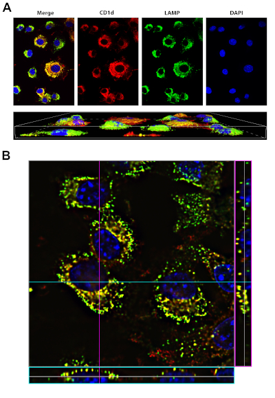
Figure 4: Staining of CD1d and LAMP1. Please click here to view a larger version of this figure.
A, top panel: LCD1 cells were fixed, permeabilized and stained with antibodies to CD1d (red) and LAMP-1 (green, a marker of the lysosomal compartment). DAPI (blue, was used to visualize the nucleus). The merge (left panel) shows that CD1d is localized in the LAMP-1 positive late endosomal/lysosomal compartment (yellow).
A, bottom panel: 3D rendering of the same cells in top panel. Images were acquired using a 40x oil-immersion objective on the Nikon Eclipse Ti, using the NIS Elements Advanced Research software.
B: 100x image of LCD1d cells stained as in A, with stack information for a particular y-coordinate (denoted by the blue line) on the bottom of the image (blue box). The stack information for a particular x-coordinate (denoted by the pink line) is shown on the right side of the image (pink box).
Confocal fluorescent staining is a relatively simple procedure that results in extremely high-quality images of specimens that are prepared in a similar way as for conventional fluorescence microscopy. In brief, samples are fixed, permeabilized, then blocked. Primary antibodies against a protein or proteins of interest are allowed to bind, then fluorophore-conjugated secondary antibodies are used to visualize the staining. Confocal fluorescence microscopy has applications in many areas of research. For example, by staining for markers of sub-cellular organelles along with a protein of interest, confocal microscopy can be used to determine the subcellular locations of diverse proteins. Compared to conventional fluorescence microscopy, confocal imaging can more effectively distinguish between cell surface and intracellular location of a protein. In addition, confocal imaging can also be used to determine whether two proteins co-localize within the cell. Although not outlined in this protocol, confocal fluorescence microscopy also can be performed on live cells to detect dynamic changes.
Video 1: Video created in NIS Elements Advanced Research software, highlighting the ability to move through the 3D rendering of the images. Please click here to view this video (Right click to download).