Fonte: Dominique R. Bollino1, Eric A. Legenzov2, Tonya J. Webb1
1 Dipartimento di Microbiologia e Immunologia, University of Maryland School of Medicine e Marlene and Stewart Greenebaum Comprehensive Cancer Center, Baltimora, Maryland 21201
2 Center for Biomedical Engineering and Technology, University of Maryland School of Medicine, Baltimora, Maryland 21201
La microscopia a fluorescenza confocale è una tecnica di imaging che consente una maggiore risoluzione ottica rispetto alla microscopia a epifluorescenza convenzionale “a campo largo”. I microscopi confocali sono in grado di ottenere una migliore risoluzione ottica x-y attraverso la “scansione laser”, in genere un insieme di specchi controllati in tensione (galvanometro o specchi “galvo”) che dirigono l’illuminazione laser a ciascun pixel del campione alla volta. Ancora più importante, i microscopi confocali raggiungono una risoluzione z-assiale superiore utilizzando un foro stenopeico per rimuovere la luce fuori fuoco proveniente da posizioni che non si trovano nel piano z in fase di scansione, consentendo così al rilevatore di raccogliere dati da un piano z specificato. A causa dell’elevata risoluzione z ottenibile in microscopia confocale, è possibile raccogliere immagini da una serie di piani z (chiamati anche z-stack) e costruire un’immagine 3D tramite software.
Prima di discutere il meccanismo di un microscopio confocale, è importante considerare come un campione interagisce con la luce. La luce è composta da fotoni, pacchetti di energia elettromagnetica. Un fotone che impaa su un campione biologico può interagire con le molecole che compongono il campione in uno dei quattro modi: 1) il fotone non interagisce e passa attraverso il campione; 2) il fotone viene riflesso/disperso; 3) il fotone viene assorbito da una molecola e l’energia assorbita viene rilasciata come calore attraverso processi noti collettivamente come decadimento non radiativo; e 4) il fotone viene assorbito e l’energia viene quindi rapidamente riemessa come fotone secondario attraverso il processo noto come fluorescenza. Una molecola la cui struttura consente l’emissione di fluorescenza è chiamata fluoroforo. La maggior parte dei campioni biologici contiene fluorofori endogeni trascurabili; pertanto i fluorofori esogeni devono essere utilizzati per evidenziare le caratteristiche di interesse nel campione. Durante la microscopia a fluorescenza, il campione viene illuminato con luce della lunghezza d’onda appropriata per l’assorbimento da parte del fluoroforo. Dopo aver assorbito un fotone, si dice che un fluoroforo sia “eccitato” e il processo di assorbimento è indicato come “eccitazione”. Quando un fluoroforo cede energia sotto forma di fotone, il processo è noto come “emissione” e il fotone emesso è chiamato fluorescenza.
Il fascio di luce utilizzato per eccitare un fluoroforo è focalizzato dalla lente obiettiva di un microscopio e converge in un “punto focale” dove è focalizzato al massimo. Oltre il punto focale la luce diverge di nuovo. I fasci in entrata e in uscita possono essere visualizzati come una coppia di coni che toccano il punto focale (vedere figura 1, pannello di sinistra). Il fenomeno della diffrazione impone un limite alla misura in cui un fascio di luce può essere focalizzato – il raggio in realtà si concentra su un punto di dimensioni finite. Due fattori determinano la dimensione del punto focale: 1) la lunghezza d’onda della luce e 2) la capacità di raccolta della luce della lente dell’obiettivo, che è caratterizzata dalla sua apertura numerica (NA). Lo “spot” focale si estende non solo nel piano x-y, ma anche nella direzione z, ed è in realtà un volume focale. Le dimensioni di questo volume focale definiscono la massima risoluzione ottenibile con l’imaging ottico. Sebbene il numero di fotoni sia maggiore all’interno del volume focale, i percorsi di luce conica sopra e sotto la messa a fuoco contengono anche una minore densità di fotoni. Qualsiasi fluoroforo nel percorso della luce può quindi essere eccitato. Nella microscopia a epifluorescenza convenzionale (a campo largo), l’emissione di fluorofori sopra e sotto il piano focale contribuisce alla fluorescenza fuori fuoco (uno “sfondo nebuloso”), che riduce la risoluzione e il contrasto dell’immagine, come dimostrato nella Figura 1, con il cubo rosso che rappresenta l’emissione di fluoroforo sopra il piano focale (stella rossa) che si traduce in fluorescenza fuori fuoco (in alto a destra). Questo problema è migliorata nella microscopia confocale, a causa dell’utilizzo di un foro stenopeico. (Figura 2, in basso a destra). Come illustrato nella Figura 3, il foro stenopeico consente alle emissioni provenienti dal punto focale di raggiungere il rilevatore (a sinistra), impedendo al contempo alla fluorescenza fuori fuoco (a destra) di raggiungere il rilevatore, migliorando così sia la risoluzione che il contrasto.
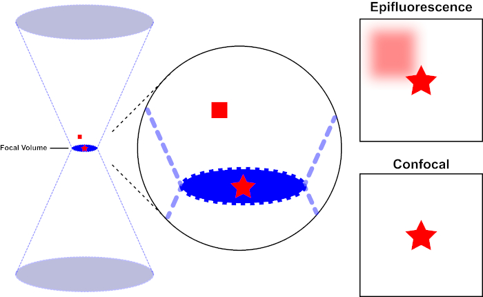
Figura 1. Risoluzione ottica dell’epifluorescenza rispetto alla microscopia confocale. Fare clic qui per visualizzare una versione più grande di questa figura.
Il fascio di luce utilizzato per eccitare un fluoroforo è focalizzato dalla lente obiettiva di un microscopio e converge a un volume focale e poi diverge (a sinistra). La stella rossa rappresenta il piano focale di un campione che viene ripreso mentre il quadrato rosso rappresenta l’emissione di fluorofori sopra il piano focale. Quando si cattura un’immagine di questo campione utilizzando un microscopio epifluorescente, l’emissione dal quadrato rosso sfocato sarà visibile e contribuirà a uno “sfondo nebuloso” (in alto a destra). I microscopi confocali hanno un foro stenopeico che impedisce il rilevamento della luce emessa al di fuori del piano focale, eliminando lo “sfondo nebuloso” (in basso a destra).

Figura 2. Effetto stenopeico in microscopia confocale. Fare clic qui per visualizzare una versione più grande di questa figura.
Sebbene la massima intensità della luce di eccitazione sia nel punto focale della lente (sinistra, ovale rosso), altre parti del campione non nel punto focale (destra, stella rossa) riceveranno luce e fluorescenza. Per evitare che la luce emessa da queste regioni fuori fuoco raggiunga il rilevatore, uno schermo con un foro stenopeico è presente davanti al rilevatore. Solo la luce a fuoco (a sinistra) emessa dal piano focale è in grado di viaggiare attraverso il foro stenopeico e raggiungere il rilevatore. La luce fuori fuoco (a destra) è bloccata con il foro stenopeico e non riesce a raggiungere il rilevatore.
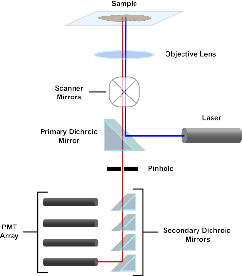
Figura 3. Componenti principali di un microscopio a scansione laser confocale. Fare clic qui per visualizzare una versione più grande di questa figura.
Per semplicità, la descrizione meccanicistica di un microscopio confocale sarà limitata a quella del Nikon Eclipse Ti A1R. Sebbene ci possano essere piccole differenze tecniche tra i diversi microscopi confocali, l’A1R funge bene da buon modello per descrivere la funzione del microscopio confocale. Il fascio di luce di eccitazione, prodotto da una serie di laser a diodi, viene riflesso dallo specchio dicroico primario nell’obiettivo, che focalizza la luce sul campione che viene ripreso. Lo specchio dicroico primario riflette selettivamente la luce di eccitazione mentre consente alla luce ad altre lunghezze d’onda di passare. La luce incontra quindi gli specchi di scansione che spazzano il fascio di luce attraverso il campione in modo x-y, illuminando un singolo(x,y)pixel alla volta. La fluorescenza emessa dai fluorofori al pixel illuminato viene raccolta dalla lente dell’obiettivo e passa attraverso lo specchio dicroico primario per raggiungere una serie di tubi fotomoltiplicatori (PMT). Gli specchi dicroici secondari dirigono la luce di emissione verso il PMT appropriato. La luce di eccitazione diffusa dal campione nell’obiettivo viene riflessa dallo specchio dicroico primario verso il campione, impedendo così di entrare nel percorso luminoso di rilevamento e raggiungere i PMT (vedere Figura 3). Ciò consente di quantificare la fluorescenza relativamente debole senza contaminazione da parte della luce diffusa dal fascio di luce di eccitazione, che è tipicamente ordini di grandezza più intenso della fluorescenza. Poiché il foro stenopeico blocca la luce dall’esterno del volume focale, la luce che arriva al rilevatore proviene da un piano zstretto e selezionato. Pertanto, le immagini possono essere raccolte da una serie di piani zadiacenti; questa serie di immagini è spesso indicata come “z-stack”. Utilizzando il software appropriato, è possibile elaborare uno z-stack per generare un’immagine 3D del campione. Un particolare vantaggio della microscopia confocale è la capacità di distinguere la localizzazione subcellulare della colorazione. Ad esempio, la differenziazione tra la colorazione di membrana dalla colorazione intracellulare, che è molto impegnativa con la microscopia a epifluorescenza convenzionale (1, 2, 3).
La preparazione del campione è un aspetto importante dell’imaging confocale. Un punto di forza delle tecniche di microscopia ottica è la flessibilità di immaginare cellule vive o fisse. Quando si tenta di produrre immagini 3D, a causa del numero di immagini che devono essere acquisite per uno z-stack, della difficoltà di mantenere la salute delle cellule e del movimento delle cellule vive e dei loro organelli, l’uso di cellule fisse è tipico. La procedura per fissare e colorare le cellule per la fluorescenza confocale è simile a quella convenzionalmente utilizzata nell’immunofluorescenza. Dopo la coltura in vetrini da camera o su coverslip, le cellule vengono fissate utilizzando la paraformaldeide per preservare la morfologia cellulare. Il legame anticorpale non specifico viene bloccato utilizzando albumina sierica bovina, latte o siero normale. Al fine di mantenere la specificità degli anticorpi secondari, la soluzione utilizzata non deve provenire dalla stessa specie in cui sono stati generati gli anticorpi primari. Le cellule vengono incubate con anticorpi primari che legano l’antigene di interesse. Quando si etichettano diversi bersagli cellulari, gli anticorpi primari devono essere derivati ciascuno da una specie diversa. Gli anticorpi che etichettano un antigene sono quindi legati da anticorpi secondari coniugati con fluoroforo. Gli anticorpi secondari coniugati con fluoroforo devono essere selezionati in modo che siano compatibili con le lunghezze d’onda dell’eccitazione laser disponibili nel microscopio confocale. Quando si visualizzano più antigeni, gli spettri di eccitazione/emissione dei fluorofori dovrebbero differire abbastanza da far sì che i loro segnali possano essere discriminati mediante analisi microscopiche. Il campione macchiato viene quindi montato su una diapositiva per l’imaging. Un mezzo di montaggio viene utilizzato per prevenire il fotosciviazione e la disidratazione del campione. Se lo si desidera, è possibile utilizzare un mezzo di montaggio contenente una controstena nucleare (ad esempio DAPI o Hoechst) (4).
Nel seguente protocollo, i fibroblasti di topo trasfettato per esprimere CD1d (LCD1) sono stati colorati con anticorpi che riconoscono CD1d e CD107a (LAMP-1). CD1d è un importante recettore simile al complesso di istocompatibilità 1 (MHC 1) presente sulla superficie delle cellule presentanti l’antigene che presenta antigeni lipidici. LAMP-1 (lysosomal associated membrane protein-1) è una proteina transmembrana presente principalmente nelle membrane liposomiali. Per una corretta presentazione dell’antigene, CD1d viene trafficato attraverso il compartimento liposomiale a basso pH, quindi LAMP-1 viene utilizzato come marcatore del compartimento liposomiale per questo protocollo. Sondando le cellule LCD1 con anti-CD1d e anti-LAMP-1 che sono state prodotte in diverse specie, gli anticorpi secondari con fluorofori unici possono essere utilizzati per determinare la localizzazione di ciascuna proteina nella cellula e se CD1d è presente nei compartimenti liposomiali positivi LAMP-1.
In this experiment, mouse fibroblasts expressing the surface glycoprotein gene CD1d were fixed, immunostained and imaged on a confocal microscope. A representative image obtained using the above protocol is shown in Figure 4. In the top panel of A, single-channel images showing the staining pattern of each individual target are presented. These images comprise a single section (slice) of the z-stack captured. The right panel shows DAPI staining of nuclei of the cells. The center panels show CD1d stained in red and LAMP-1, a lysosomal marker, stained in green. The left panel is a composite image where the three different channels are merged. The appearance of yellow results from overlap of the red and green channels, and indicates an area where CD1d and LAMP-1 are co-localized. The results of the staining confirm that CD1d is localized in the LAMP-1+ endosomal compartments. There are also areas where only one color is present, which indicates the presence of CD1d or LAMP-1 without co-localization. The bottom panel of A shows a 3D rendering of the cells constructed from images captured in the z-stack.
Panel B shows a slice out of the z-stack at 100x magnification demonstrating the expression patterns of these two proteins in greater detail. The pink outlined box on the right side of the image displays the cross section of the x-coordinate designated by the pink line in the image, which represents the side view at the pink line. Similarly, the blue outlined box on the bottom of the image shows the cross section of the y-coordinate designated by the blue line in the image, which represents the front view at the blue line. The 3D rendering of the z-stack image enables users to view the image in 3D, visualizing all the x, y and z planes.
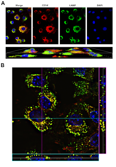
Figure 4: Staining of CD1d and LAMP1. Please click here to view a larger version of this figure.
A, top panel: LCD1 cells were fixed, permeabilized and stained with antibodies to CD1d (red) and LAMP-1 (green, a marker of the lysosomal compartment). DAPI (blue, was used to visualize the nucleus). The merge (left panel) shows that CD1d is localized in the LAMP-1 positive late endosomal/lysosomal compartment (yellow).
A, bottom panel: 3D rendering of the same cells in top panel. Images were acquired using a 40x oil-immersion objective on the Nikon Eclipse Ti, using the NIS Elements Advanced Research software.
B: 100x image of LCD1d cells stained as in A, with stack information for a particular y-coordinate (denoted by the blue line) on the bottom of the image (blue box). The stack information for a particular x-coordinate (denoted by the pink line) is shown on the right side of the image (pink box).
Confocal fluorescent staining is a relatively simple procedure that results in extremely high-quality images of specimens that are prepared in a similar way as for conventional fluorescence microscopy. In brief, samples are fixed, permeabilized, then blocked. Primary antibodies against a protein or proteins of interest are allowed to bind, then fluorophore-conjugated secondary antibodies are used to visualize the staining. Confocal fluorescence microscopy has applications in many areas of research. For example, by staining for markers of sub-cellular organelles along with a protein of interest, confocal microscopy can be used to determine the subcellular locations of diverse proteins. Compared to conventional fluorescence microscopy, confocal imaging can more effectively distinguish between cell surface and intracellular location of a protein. In addition, confocal imaging can also be used to determine whether two proteins co-localize within the cell. Although not outlined in this protocol, confocal fluorescence microscopy also can be performed on live cells to detect dynamic changes.
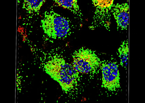
Video 1: Video created in NIS Elements Advanced Research software, highlighting the ability to move through the 3D rendering of the images. Please click here to view this video (Right click to download).