Fonte: Dominique R. Bollino1, Eric A. Legenzov2, Tonya J. Webb1
1 Departamento de Microbiologia e Imunologia, Faculdade de Medicina da Universidade de Maryland e o Centro de Câncer Integral Marlene e Stewart Greenebaum, Baltimore, Maryland 21201
2 Center for Biomedical Engineering and Technology, University of Maryland School of Medicine, Baltimore, Maryland 21201
A microscopia de fluorescência confocal é uma técnica de imagem que permite maior resolução óptica em comparação com a microscopia convencional de epifluorescência “campo largo”. Microscópios confocal são capazes de obter uma resolução óptica x-y melhorada através da “varredura a laser”, tipicamente um conjunto de espelhos controlados por tensão (espelhos galvanômetros ou “galvo”) que direcionam a iluminação a laser para cada pixel da amostra de cada vez. Mais importante, os microscópios confocal atingem uma resolução z-axial superior usando um pinhole para remover a luz de foco originária de locais que não estão no plano z que está sendo escaneado, permitindo assim que o detector colete dados de um z-plane especificado. Devido à alta resolução z alcançável na microscopia confocal, é possível coletar imagens de uma série de z-planes (também chamado de z-stack) e construir uma imagem 3D através de software.
Antes de discutir o mecanismo de um microscópio confocal, é importante considerar como uma amostra interage com a luz. A luz é composta de fótons, pacotes de energia eletromagnética. Um fóton que implica em uma amostra biológica pode interagir com as moléculas que compõem a amostra de uma das quatro maneiras: 1) o fóton não interage e passa pela amostra; 2) o fóton é refletido/espalhado; 3) o fóton é absorvido por uma molécula e a energia absorvida é liberada como calor através de processos coletivamente conhecidos como decadência nãoraditória; e 4) o fóton é absorvido e a energia é rapidamente reemitida como um fóton secundário através do processo conhecido como fluorescência. Uma molécula cuja estrutura permite a emissão de fluorescência é chamada de fluorófora. A maioria das amostras biológicas contém fluoroforos endógenos insignificantes; portanto, fluoroforos exógenos devem ser usados para destacar características de interesse na amostra. Durante a microscopia de fluorescência, a amostra é iluminada com luz do comprimento de onda apropriado para absorção pelo fluoróforo. Ao absorver um fóton, diz-se que um fluoróforo está “animado” e o processo de absorção é chamado de “excitação”. Quando um fluoróforo abre mão de energia na forma de um fóton, o processo é conhecido como “emissão”, e o fóton emitido é chamado de fluorescência.
O feixe de luz usado para excitar um fluoróforo é focado pela lente objetiva de um microscópio e converge em um “ponto focal” onde é extremamente focado. Além do ponto focal, a luz novamente diverge. Os feixes de entrada e saída podem ser visualizados como um par de cones tocando no ponto focal (ver Figura 1, painel esquerdo). O fenômeno da difração impõe um limite de quão firmemente um feixe de luz pode ser focado – o feixe realmente se concentra em um ponto de tamanho finito. Dois fatores determinam o tamanho da mancha focal: 1) o comprimento de onda da luz, e 2) a capacidade de captação de luz da lente objetiva, que é caracterizada por sua abertura numérica (NA). O “ponto” focal se estende não só no plano x-y, mas também na direção z, e é na realidade um volume focal. As dimensões deste volume focal definem a resolução máxima alcançável por imagem óptica. Embora o número de fótons seja maior dentro do volume focal, os caminhos de luz cônica acima e abaixo do foco também contêm uma menor densidade de fótons. Qualquer fluoróforo no caminho da luz pode, assim, ser animado. Na microscopia convencional (campo largo), a emissão de fluoroforos acima e abaixo do plano focal contribuem com fluorescência fora de foco (um “fundo nebuloso”), o que reduz a resolução e o contraste da imagem, como demonstrado na Figura 1, com o cubo vermelho representando a emissão de fluorhoreo acima do plano focal (estrela vermelha) que resulta em fluorescência fora de foco (superior à direita). Este problema é amenizado em microscopia confocal, devido à utilização de um orifício. (Figura 2, inferior direito). Como descrito na Figura 3, o orifício permite que as emissões originárias do local focal cheguem ao detector (esquerda), enquanto bloqueiam a fluorescência fora de foco (direita) de atingir o detector, melhorando assim tanto a resolução quanto o contraste.
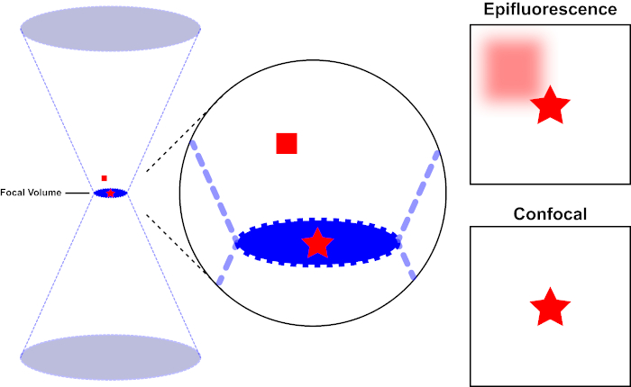
Figura 1. Resolução óptica de epifluorescência versus microscopia confocal. Clique aqui para ver uma versão maior desta figura.
O feixe de luz usado para excitar um fluoróforo é focado pela lente objetiva de um microscópio e converge em um volume focal e, em seguida, diverge (esquerda). A estrela vermelha representa o plano focal de uma amostra que está sendo imagen, enquanto o quadrado vermelho representa a emissão de fluoróforo acima do plano focal. Ao capturar uma imagem desta amostra usando um microscópio epifluorescente, a emissão do quadrado vermelho fora de foco será visível e contribuirá para um “fundo nebuloso” (canto superior direito). Os microscópios confocal têm um orifício que impede a detecção de luz emitida fora do plano focal, eliminando o “fundo nebuloso” (inferior direito).

Figura 2. Efeito pinhole na microscopia confocal. Clique aqui para ver uma versão maior desta figura.
Embora a maior intensidade da luz de excitação esteja no ponto focal da lente (esquerda, oval vermelho), outras partes da amostra não no ponto focal (direita, estrela vermelha) receberão luz e fluoresce. Para evitar que a luz emitida dessas regiões fora de foco chegue ao detector, uma tela com um orifício está presente na frente do detector. Apenas a luz em foco (esquerda) emitindo do plano focal é capaz de viajar através do orifício e alcançar o detector. A luz fora de foco (à direita) é bloqueada com o orifício e não alcança o detector.
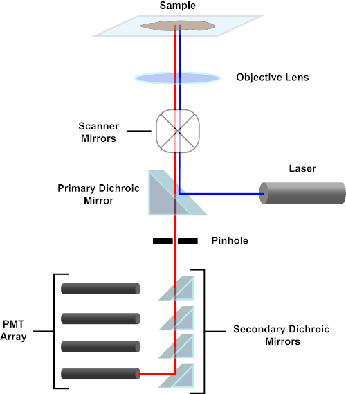
Figura 3. Principais componentes de um microscópio de varredura a laser confocal. Clique aqui para ver uma versão maior desta figura.
Por uma questão de simplicidade, a descrição mecanicista de um microscópio confocal será limitada à do Nikon Eclipse Ti A1R. Embora possa haver pequenas diferenças técnicas entre diferentes microscópios confocal, o A1R serve bem como um bom modelo para descrever a função de microscópio confocal. O feixe de luz de excitação, produzido por uma matriz de lasers de diodo, é refletido pelo espelho dicroico primário no objetivo, que foca a luz no espécime que está sendo imageado. O espelho dicroico primário reflete seletivamente a luz de excitação, permitindo que a luz em outros comprimentos de onda passe. A luz então encontra os espelhos de varredura que varrem o feixe de luz através do espécime de uma maneira x-y, iluminando um único (x,y) pixel de cada vez. A fluorescência emitida por fluoroforos no pixel iluminado é coletada pela lente objetiva e passa pelo espelhodicrómico primário para alcançar uma matriz de tubos fotomultiplier (PMTs). Espelhos dicroicos secundários direcionam a luz de emissão para o PMT apropriado. A luz de excitação espalhada pela amostra de volta ao objetivo é refletida pelo espelho dirítmico primário de volta para o espécime, e assim impedido de entrar no caminho da luz de detecção e chegar aos PMTs (ver Figura 3). Isso permite que a fluorescência relativamente fraca seja quantificada sem contaminação pela luz espalhada do feixe de luz de excitação, que é tipicamente ordens de magnitude mais intensas do que a fluorescência. Como o orifício bloqueia a luz de fora do volume focal, a luz que chega ao detector vem de um plano Zestreito e selecionado. Portanto, as imagens podem ser coletadas a partir de uma série de z-planesadjacentes; esta série de imagens é frequentemente referida como uma “pilha de z”. Usando o software apropriado, uma pilha zpode ser processada para gerar uma imagem 3D do espécime. Uma vantagem particular da microscopia confocal é a capacidade de distinguir a localização subcelular da coloração. Por exemplo, a diferenciação entre a coloração da membrana a partir da coloração intracelular, que é muito desafiadora com a microscopia de epifluorescência convencional (1, 2, 3).
A preparação da amostra é uma faceta importante da imagem confocal. Uma força das técnicas ópticas de microscopia é a flexibilidade para imagem de células vivas ou fixas. Ao tentar produzir imagens 3D, devido ao número de imagens que devem ser adquiridas para uma pilha z, a dificuldade de manter a saúde celular, e o movimento de células vivas e suas organelas, o uso de células fixas é típico. O procedimento para fixação e coloração de células para fluorescência confocal é semelhante ao convencionalmente utilizado na imunofluorescência. Após a cultura em slides de câmara ou em deslizamentos de cobertura, as células são fixadas usando paraformaldeído para preservar a morfologia celular. A ligação de anticorpos não específicos é bloqueada usando albumina de soro bovino, leite ou soro normal. Para manter a especificidade dos anticorpos secundários, a solução utilizada não deve ser originária da mesma espécie em que os anticorpos primários foram gerados. As células são incubadas com anticorpos primários que ligam o antígeno de interesse. Ao rotular vários alvos celulares, os anticorpos primários devem ser derivados de uma espécie diferente. Anticorpos que marcam um antígeno são então ligados por anticorpos secundários conjugados por fluoróforo. Os anticorpos secundários conjugados por fluoróforo devem ser selecionados para que sejam compatíveis com os comprimentos de onda da excitação a laser disponíveis no microscópio confocal. Ao visualizar múltiplos antígenos, os espectros de excitação/emissão dos fluoroforos devem diferir o suficiente para que seus sinais possam ser discriminados pela análise microscópica. O espécime manchado é então montado em um slide para imagens. Um meio de montagem é usado para evitar fotobleaching e desidratação da amostra. Se desejar, um meio de montagem contendo uma contra-mancha nuclear (por exemplo, DAPI ou Hoechst) pode ser usado (4).
No protocolo a seguir, os fibroblastos de camundongos transfectados para expressar CD1d (LCD1) foram manchados com anticorpos que reconhecem CD1d e CD107a (LAMP-1). CD1d é um grande receptor do complexo de histocompatibilidade 1 (MHC 1) presente na superfície de células presentes de antígenos que apresentam antígenos lipídicos. LAMP-1 (proteína de membrana associada à linsósomal-1) é uma proteína transmembrana presente principalmente em membranas lysosômicas. Para apresentação adequada de antígeno, o CD1d é traficado através do compartimento lyososômico de pH baixo, por isso o LAMP-1 está sendo usado como um marcador do compartimento lysosomal para este protocolo. Ao sondar as células LCD1 com anti-CD1d e anti-LAMP-1 que foram produzidas em diferentes espécies, anticorpos secundários com fluoroforos únicos podem ser usados para determinar a localização de cada proteína na célula e se o CD1d está presente nos compartimentos lisesosmal positivos da LAMP-1.
In this experiment, mouse fibroblasts expressing the surface glycoprotein gene CD1d were fixed, immunostained and imaged on a confocal microscope. A representative image obtained using the above protocol is shown in Figure 4. In the top panel of A, single-channel images showing the staining pattern of each individual target are presented. These images comprise a single section (slice) of the z-stack captured. The right panel shows DAPI staining of nuclei of the cells. The center panels show CD1d stained in red and LAMP-1, a lysosomal marker, stained in green. The left panel is a composite image where the three different channels are merged. The appearance of yellow results from overlap of the red and green channels, and indicates an area where CD1d and LAMP-1 are co-localized. The results of the staining confirm that CD1d is localized in the LAMP-1+ endosomal compartments. There are also areas where only one color is present, which indicates the presence of CD1d or LAMP-1 without co-localization. The bottom panel of A shows a 3D rendering of the cells constructed from images captured in the z-stack.
Panel B shows a slice out of the z-stack at 100x magnification demonstrating the expression patterns of these two proteins in greater detail. The pink outlined box on the right side of the image displays the cross section of the x-coordinate designated by the pink line in the image, which represents the side view at the pink line. Similarly, the blue outlined box on the bottom of the image shows the cross section of the y-coordinate designated by the blue line in the image, which represents the front view at the blue line. The 3D rendering of the z-stack image enables users to view the image in 3D, visualizing all the x, y and z planes.
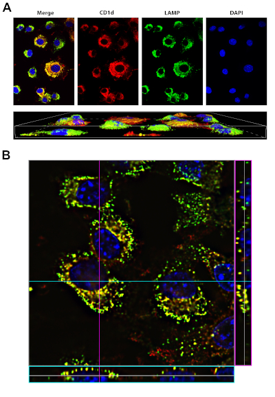
Figure 4: Staining of CD1d and LAMP1. Please click here to view a larger version of this figure.
A, top panel: LCD1 cells were fixed, permeabilized and stained with antibodies to CD1d (red) and LAMP-1 (green, a marker of the lysosomal compartment). DAPI (blue, was used to visualize the nucleus). The merge (left panel) shows that CD1d is localized in the LAMP-1 positive late endosomal/lysosomal compartment (yellow).
A, bottom panel: 3D rendering of the same cells in top panel. Images were acquired using a 40x oil-immersion objective on the Nikon Eclipse Ti, using the NIS Elements Advanced Research software.
B: 100x image of LCD1d cells stained as in A, with stack information for a particular y-coordinate (denoted by the blue line) on the bottom of the image (blue box). The stack information for a particular x-coordinate (denoted by the pink line) is shown on the right side of the image (pink box).
Confocal fluorescent staining is a relatively simple procedure that results in extremely high-quality images of specimens that are prepared in a similar way as for conventional fluorescence microscopy. In brief, samples are fixed, permeabilized, then blocked. Primary antibodies against a protein or proteins of interest are allowed to bind, then fluorophore-conjugated secondary antibodies are used to visualize the staining. Confocal fluorescence microscopy has applications in many areas of research. For example, by staining for markers of sub-cellular organelles along with a protein of interest, confocal microscopy can be used to determine the subcellular locations of diverse proteins. Compared to conventional fluorescence microscopy, confocal imaging can more effectively distinguish between cell surface and intracellular location of a protein. In addition, confocal imaging can also be used to determine whether two proteins co-localize within the cell. Although not outlined in this protocol, confocal fluorescence microscopy also can be performed on live cells to detect dynamic changes.
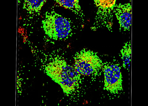
Video 1: Video created in NIS Elements Advanced Research software, highlighting the ability to move through the 3D rendering of the images. Please click here to view this video (Right click to download).